Chapter 1 Statistics Refresher
This chapter covers statistical concepts that are central in any statistical analysis. We will use the example of dice rolls to develop an intuition for these concepts.
1.1 Lingo: Estimators, Estimates and all that
In most (if not all) statistical analyses, we want to learn something about a population of interest. The population of interest does not need to be the actual population of a country or the world, but it can also be a very specific population such as all students in this course, all people below age 25, all countries (or only those with a GDP less than 20k€), etc. However, using the entire population for an analysis is usually not practical and often impossible. For example, if you were to do a blood test with the entire population – all the blood in a patient’s body – you would get the best possible information about the population of interest, but you can also be sure that the patient won’t survive the test. For this reason, blood tests are based on a small sample of blood. As we will learn, much can be learned from relatively small samples about the population.
Within the population of interest, we are typically interested in a particular statistic – which is sometimes called target parameter or quantity of interest or population statistic or estimand. Your doctor wants to know the concentration of certain biomarkers in all your blood cells. As a policy analyst, we want to know the impact of childcare subsidies on child development, etc. These are examples of population statistics we are interested in.
If our analysis is based on a sample rather than the population, we say that we estimate these population statistics. This means that we compute the same statistic in our sample. The procedure we use to do this is called estimator and the result, i.e. the statistic computed from the sample, is called estimate. Once we obtained an estimate, we use insights from statistics to assess how much we can learn from this estimate about the population statistic we are interested in.
For example, we may be interested in the population mean \(\mu_Y\). We can draw a random sample of size \(n\) from the population and estimate the population mean using the formula for the sample mean,
\[\begin{equation} \overline{Y}=\frac{1}{n}\displaystyle\sum_{i=1}^n Y_i. \tag{1.1} \end{equation}\]
The formula in Equation ((eq:mean)) is the estimator for the population mean \(\mu_Y\). If we apply the estimator to a particular sample \(s\), we obtain an estimate \(\overline{Y_s}\)for the sample \(s\). If we were to draw another sample \(t \neq s\), we use the same estimator but obtain a different estimate \(\overline{Y_t}\).
Definition: Estimator and Estimate
An estimator is a procedure that is used for calculating an estimate for a quantity of of interest based on a sample from the population of interest.
In plain English: An estimator is to an estimate what a recipe is to a cake. Suppose we want to bake a chocolate cake (that’s the quantity, or in that case rather the object of interest). We then use recipe that tells us how we convert the ingredients into a chocolate cake. The recipe is the equivalent of the estimator. When we do this, we hopefully get a tasty chocolate cake, which is the estimate. But every time we do this, we get a cake that tastes slightly different. It’s the same with estimators. Not that we know what they taste like, but we get a different estimate every time we apply the same estimator to a different sample.
1.2 The Sampling Distribution
The sampling distribution is central to any statistical analysis. After all, we typically cannot analyse the entire population of interest but have to draw inference from a smaller random sample. As we will see, there is a lot that can be learned about the population even from a medium-sized random sample. However, an analysis that is based on random sampling comes with the challenge that every random sample will yield different estimates. Suppose we wanted to estimate the mean height of students at UCD. If we draw five students at random and calculate the mean height of these students, we may end up with an estimate that is larger than the true mean – if we happen to disproportionately sample taller students – or smaller than the true mean – if we happen to disproportionately sample shorter students. If we draw many such samples and compute the mean in each sample, we will likely get a different mean height in each sample. The distribution of these means is called the sampling distribution.
Definition: Sampling Distribution
Wikipedia says: A sampling distribution or finite-sample distribution is the probability distribution of a given random-sample-based statistic.
In plain English: Suppose we draw many random samples and in each sample we compute the same statistic (for example the mean, variance, minimum or maximum). The distribution of these statistics across all samples is called the sampling distribution.
When students encounter the sampling distribution for the first time, they tend to struggle with this concept. To illustrate what the sampling distribution is, where it comes from and what it is useful for, we will consider dice rolls. If we have a fair dice, the expected number of points is 3.5. This is the case because each side comes up with a probability of \(1/6\), and thus the (population) mean is
\[\begin{equation*} \mu_Y=\frac{1}{6}\times \left(1 + 2 + 3 + 4 + 5 + 6\right)=3.5. \end{equation*}\]
This mean is what we will get if we roll a dice an infinite number of times and calculate the mean across all rolls. But that’s a theoretical quantity. No one can actually roll a dice so many times. The real question here is what happens if we roll a dice a finite number of times and take the mean. In that case we need to compute the sample mean \(\overline{Y}\) over all \(i \in \{1, \dots, n\}\) dice rolls
\[\begin{equation*} \overline{Y}=\frac{1}{n}\displaystyle\sum_{i=1}^n Y_i, \end{equation*}\]
whereby \(Y_i\) are the points from an individual diceroll.
\[\\[0.3cm]\]
We can also compute the population variance of a dice roll for \(Y \in \{1,2,3,4,5,6\}\) (remember: population here means an infinite number of dice rolls):
\[\begin{equation*} \sigma_Y^2=\frac{1}{6} \displaystyle\sum_{i=1}^6 (Y_i-\mu_Y)^2=\approx 2.92. \end{equation*}\]
Need a refresher of expected value and variance? Check out this video: https://www.youtube.com/watch?v=OvTEhNL96v0.
Sampling distribution in very small samples
Let’s start with a small sample size: we roll two dice, compute the mean, roll two dice, compute the mean, and so on. Figure 1.1 shows the result of this exercise with 200 samples (i.e. 200 times we roll two dice and compute the mean). The orange panels at the top show the points of the two dice. With every sample of size two, we add a new mean to the distribution shown in the panel at the bottom (the grey line highlights where in the distribution the new mean falls).
Figure 1.1: Sampling Distribution: Two Dice Rolls per Sample
The distribution that emerges – the sampling distribution – is quite interesting. The distribution seems to be fairly symmetric around the population mean of 3.5, and there are more samples with means between 2 and 4 and fewer with means smaller than 2 or larger than 4. This distribution should not come as a surprise because there are more combinations that yield a sample mean of 3.5 – \(\{3,4\}\), \(\{2,5\}\), \(\{1,6\}\) all yield a sample mean of 3.5, whereas a sample mean of 1 can only occur with the combination \(\{1,1\}\).
Sampling distribution in larger samples
Now consider slightly larger samples. In Figure 1.2 the sample size is ten dice rolls.
Figure 1.2: Sampling Distribution: 10 Dice Rolls per Sample
As was the case with samples of two dice rolls, we get a sampling distribution that is roughly symmetric around 3.5 and has a bell shape. What is different is that the distribution is a lot tighter around 3.5, which means that there are fewer extreme values than with samples of two dice. This should not be surprising. Consider a sample mean of 1, which only occurs if all dice yield one point. When we roll two dice, it is a lot more likely to have all ones than when we roll ten dice.
In Figure 1.3 we go even further and roll 100 dice at a time. Think about this like us pouring a bucket with 100 dice on the floor, calculating the mean, putting the dice back into the bucket, and starting again. Luckily, we can do this on a computer and don’t have to waste our time returning dice to a bucket.
Figure 1.3: Sampling Distribution: 100 Dice Rolls per Sample
Again, the same picture emerges, namely a bell-shaped sampling distribution that is centered on the population mean of 3.5. With a sample size of 100, almost all samples have a mean close to 3.5. And if we were to increase the sample size even further, the sampling distribution would be even tighter around the population mean of 3.5.
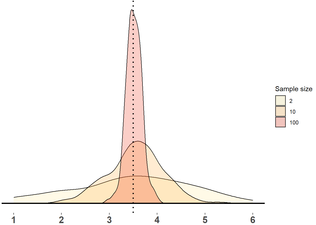
Figure 1.4: Sampling Distribution of Means (2, 10, 100 dice rolls, 200 samples each)
In Figure 1.4, we can see the histograms of the three sampling distributions. The center of all distributions is close to the expected value of \(3.5\). The distribution of the smallest sample size (2 dice rolls) is very wide whereas the distribution of samples with 100 dice rolls is fairly tight.
Key Observation
As the sample size \(n\) increases
- the mean of each sample gets closer to the expected value of \(3.5\)
- the sampling distribution of the means becomes tighter around the expected value of \(3.5\)
Explanation
With a small sample size \(n\), any particular sample may be very different from the population (where each side of the dice is equally likely to occur). We may have samples with only ones or only sixes. As the sample size \(n\) increases each individual sample looks more and more similar to the population and, thus, the sample mean becomes more similar to the population mean. This means that if we have a larger sample, we can be more confident that this sample can teach us something about the population.
\[\\[0.3cm]\]
The question is when is a sample large enough? The answer to this question unfortunately is it depends. We will later learn that samples greater than \(30\) tend to have favourable properties, but in empirical applications we would need much greater samples than that.
Sampling Distribution: Bottom Line
If we draw many random samples from a population and calculate a statistic in each random sample (such as the mean, variance, or the correlation between two variables), we will get a different value for this statistic in each sample. The distribution of these statistics is called the sampling distribution. If we have true random sampling, the sampling distribution of the mean has the following properties (for an infinite number of samples of size \(n\)):
- Sampling mean: \(E(\overline{Y})=\mu_Y\)
- Sampling variance \(Var(\overline{Y})=\frac{\sigma_Y^2}{n}\).
These properties are very useful for statistical analysis because they tell us that the sampling distribution of the mean always follows the same logic regardless whether the underlying variable is points of a dice roll or a coin flip, a person’s height, IQ, or wage. As long as we draw random samples, we know what the mean and variance of the sampling distribution look like.
1.3 The Law of Large Numbers and Consistency of an Estimator
What we observed in Figure 1.4 is the result of the Law of Large Numbers (LLN). According to the LLN, if we take an infinite number of random samples and take the sample mean \(\overline{Y}\) in each sample, then the average of all sample means, \(E(\overline{Y})\) converges to the true population mean \(\mu_Y\).
We can see this in Figure 1.4. Even with 200 small samples of size 2, the mean of the distribution is close to 3.5. If we were to draw more samples, it would get even closer to the population mean of 3.5. The LLN also implies that as the sample size \(n\) increases, each sample mean has a higher probability of being close to the population mean \(\mu_Y\). We can see this in Figure 1.4: the larger \(n\) is, the tigther is the distribution around the population mean of 3.5. If the sample was infinitely large, the distribution would collapse onto the vertical line at the population mean of 3.5.
Figure 1.5: Illustration of the LLN
Figure 1.5 illustrates the LLN based on dice rolls with sample sizes 2, 10, 50, 100 and 1000. Each dot is a sample mean, and if two samples have a similar mean we draw dots next to each other. For each sample size, we draw 200 samples. Again, we can make two observations that reflect the LLN:
- no matter what the sample size is, the mean of the distribution is close to the population mean (grey line). You can see this because all distributions are roughly symmetric around 3.5.
- As the sample size gets larger, the individual sample means are getting closer to the population mean, i.e. the distribution becomes tighter around the population mean.
1.4 The Central Limit Theorem
So far, we have established what the mean and variance of the sampling distribution is. But we can go even a step further and determine the shape of the distribution. To do that, we make use of the Central Limit Theorem (CLT).
Definition: Central Limit Theorem
Wikipedia says: The central limit theorem (CLT) establishes that, in many situations, when independent random variables are summed up, their properly normalized sum tends toward a normal distribution even if the original variables themselves are not normally distributed..
In plain English: Suppose we draw many random samples and in each sample we compute the mean. If the sample size is large enough, the sampling distribution is approximately normal (this holds for the mean and many other interesting statistics but there are some statistics where the CLT doesn’t hold.)
Formally, for the sampling distribution of \(\overline{Y}\) the CLT implies
\[\begin{equation*} \overline{Y} \sim N(\mu_Y, sd=\frac{\sigma_Y}{\sqrt{n}}), \end{equation*}\]
that is, the sample means are normally distributed with mean \(\mu_Y\) and standard deviation \(\sigma_Y/\sqrt{n}\).
CLT Animations
To get a feel for the implications of the Central Limit Theorem, let’s look at some animations. Let’s start with a very small sample size (n=2) in Figure (fig:clt2). With every sample of two dice rolls, we add the mean to the distribution. The histogram shows the relative frequency of each value on the x-axis (i.e. a percentage). For example, if the first mean is 3, then the bin at 3 shows a relative frequency of 100%. If the second sample mean is 5, we add this to the histogram, and we now have a relative frequency of 50% at 3 and 50% at 5. We do this 200 times and see to what extent the histogram converges to the normal distribution.
Figure 1.6: CLT: samples of 2 dice rolls
As we can see, the histogram does not converge to the normal distribution. It is roughly symmetric and bell-shaped but does not follow a normal distribution.
In Figure (fig:clt10), we consider sample sizes of 10 and 20, respectively. In both cases the histogram moves closer to a normal distribution. Statistical theory tells us that a sample size of 20 is still too small to assume normality. A rule of thumb is that a sample should be larger than 30 observations to justify applying a normal distribution.
In Figure (fig:clt50) we see an animation with samples of 50 dice rolls. Note that the range on the x-axis is narrower here. As we add more and more samples, the histogram gets very close to a normal distribution.
Figure 1.7: CLT: samples of 50 dice rolls
What is the CLT Useful for?
We want to learn something about the population but typically we can only work with a sample. Collecting samples is often expensive, which means that we often only have one sample. If we want to know how much we can learn from this one sample about the population, we need to know what the sampling distribution looks like. This is entirely hypothetical: if we could draw many more samples from the same population, what would the sampling distribution look like? The Central Limit Theorem, along with the Law of Large Numbers can help us make sense of the sampling distribution. We know that its mean coincides with the population mean and we know that it is approximately normally distributed with variance \(\sigma_Y/\sqrt{n}\).
Most students do not fully embrace how important this insight is and why the CLT makes our life so much easier. No matter what the distribution of \(Y\) is, that is, no matter what context or research question we study, thanks to the CLT we always know what the sampling distribution looks like. This means that we can use the same statistical analysis tools no matter what population we study. What we typically do is “standardise” the sampling distribution such that the standardised distribution is normal with mean zero and standard deviation one. We do this by subtracting the population mean and dividing by the standard deviation,
\[\begin{equation*} \frac{\overline{Y}-\mu_Y}{\sigma_Y/(\sqrt{n})} \sim N(0,1). \end{equation*}\]
When we “standardise” \(\overline{Y}\), we ensure that all the sampling distributions have mean zero and a standard deviation of 1, regardless of the characteristics of the underlying random variable \(Y\) and the sample size. The reason for doing this is a practical one. If we did not standardise \(\overline{Y}\), we would have to apply a different normal distribution – with a different mean and variance – in every analysis. By standardising, we can move this part to auto-pilot. We can use the same standard normal distribution no matter what we study.
Figure (fig:cltall) compares the sampling distribution of dice rolls with varying sample sizes to a normal distribution, N(0,1). Each picture shows the distribution of 1,000 samples of a given size, ranging from n=2 to n=200. Once we have sample sizes of 100 and larger, the histogram gets very close to a normal distribution and it would even get closer if we plotted more than 1,000 samples.

Figure 1.8: CLT: sampling distribution vs. N(0,1)